

Machine learning is a subfield of artificial intelligence where computers learn patterns from data and improve their performance on tasks over time without being explicitly programmed for every rule. Instead of following rigid human-written instructions, algorithms build mathematical models from sample inputs to make predictions or decisions on unseen data.
Setting Up the Simple Model
Imagine we have an input feature x, a true target value y, and a single model parameter (weight) w.
The Prediction: the model predicts
by multiplying the input by the weight:
The Loss Function (for a single data point): As it is noted, the squared error is:
When we have a dataset with N samples, the total loss across the entire dataset is called the Mean Squared Error (MSE) cost function J(w):
The Parabolic Landscape
Because J(w) squares the term (y – wx), if we plot J(w) on the vertical axis against different possible values of w on the horizontal axis, the resulting graph forms a convex parabola (a bowl-shaped curve).
If w is too high, predictions overshoot. If w is too low, predictions undershoot. Both of the time
grows large.
At the optimal value of w, the error is minimized at the bottom of the bowl.
Finding the Minimum via Differentiation (The Slope)
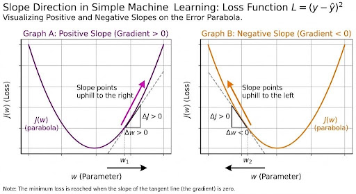
At the very bottom (the minimum error point), the slope of the tangent to the curve is zero.
To find this slope mathematically, we take the derivative of the cost function J(w) with respect to our parameter w using calculus (specifically, the power rule and chain rule):
This derivative
is the gradient. It tells you two critical things at any given point w:
1. Magnitude: How steep the slope is (how far off we are from the minimum).
2. Direction: Whether the slope is positive (pointing uphill to the right) or negative (pointing uphill to the left).
Solving the Minimum: Analytical vs. Iterative
Method A: Setting the Slope to Zero (Analytical Solution)
For simple linear equations, you can solve for the optimal w directly by setting the derivative to zero:
Solving this yields a direct algebraic formula for w. However, as machine learning models grow to billions of parameters, solving this algebraically becomes computationally impossible.
Method B: Gradient Descent (Iterative Solution)
This is where Gradient Descent comes in. Instead of solving it all at once, the model walks down the parabola step-by-step:
a. Start with a random initial guess for w.
b. Compute the gradient dJ/dw at that point.
c. Update w by taking a small step in the opposite direction of the slope:
(where α is the learning rate, controlling the size of the step).
d. Repeat this loop until the gradient approaches zero, meaning the model has reached the bottom of the parabola.
From Training to AI
The Trained Model: Once gradient descent finishes, the parameter w is locked in. The learning phase is over.
Inference: When new data x arrives, the trained model instantly computes
using that finalized weight.
Scaling to AI: When you scale this basic loop – from one weight w and a simple line to millions or billions of parameters (w1, w2, w3 etc) operating across massive neural networks and petabytes of data – you transition from simple mathematical optimization into modern Artificial Intelligence.